Sent from my ipod

Data Analysis Of Crossfit.com Workouts

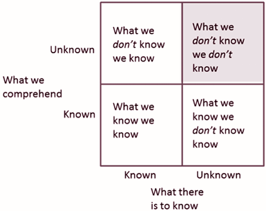
Exploring data without knowing what you are looking for allows you to find results that you didn’t know existed. Below is a chart from business school 101. The top right quandrant is seldom explored by companies that are not established as data-driven companies.

The interwebs does a great job of explaining concepts, but not so much of explaining approaches to solve a type of problem. My goal is to show you how I approach exploratory data analysis problems and leave you with a set of strategies and tools. At the very least, it will help you get started in the right direction.

Finding data to explore

The ongoing data revolution has driven plenty of organizations to make their data available publicly. A few examples are here, here, here and here.

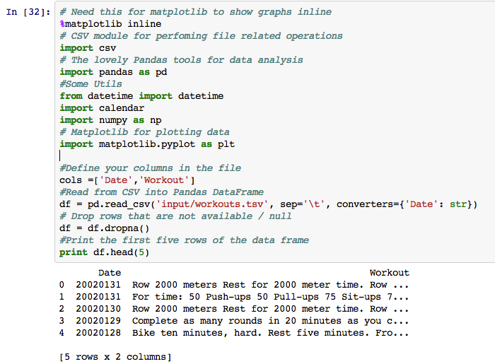
For this post, let’s pick data that we previously scraped in this post. If you haven’t read it already, I recommend you do - for context. We ended up with a tab separated file which has all the workouts scraped from the Crossfit.com website from the year 2002 to 2013. You can find a link to the file here.

Sidenote : My liking Crossfit has got nothing to do with this dataset. OK, maybe it does. A little. I wanted a practical application and this data was handy. That’s it.

Before I wrote this post, I had no idea what I wanted from this analysis. I simply felt that there was something hidden in the data.

Picking your tools

The data science / analytics space is in such flux that there are no tools that are clear winners yet. ‘R’ used to be the go-to data analysis environment. Although there are plenty of packages available for R, Python is flexible across platforms, has a great ecosystem, many applications and a huge selection of libraries.

For this analysis, we’ll use the following tools:

1. Python
2. Pandas
3. Open Refine
4. IPython notebook

I have a brief description and installation instructions for tools 1, 2 and 4 in the my previous post here. Open Refine is a UI driven open source project that allows you to clean up messy data, especially the type of data you get from web scraping. You can find installation instructions here.

Viewing your data

Although the data can be viewed in a plain Notepad or Excel, you want a tool in which you can experiment and immediately see the results. This is where the IPython Notebook shines. It is an interactive web interface that allows you to interface with your data, one step at a time.

I’ll have all this code available on Github, along with a sample IPython Notebook, so just follow along.

Sanitize your data

I use Open Refine to deal with all sought of messy data. The usual suspects are:

1. Leading or trailing white spaces
2. Control characters
3. Converting all your text to a single case
4. Removing duplicates

Looking at the example below, here are two phrases that mean the same thing, but could be typed in many different ways:

Open Refine does a good job of combining these type of phrases into one representation. The primary concept used under the hood is called Key Collision. If you want to understand one way to apply a key collision method, fingerprinting is the most basic of all. The Open Refine docs do a great job of explaining it.

In order to get your data into Open Refine, let’s export the data from Pandas in a CSV format.

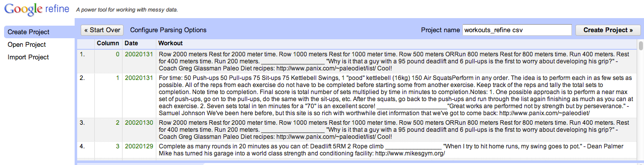
Import the file you exported from Pandas into Open Refine

Cluster all the workouts, which will give you the option to merge the similar data using the fingerprinting method.

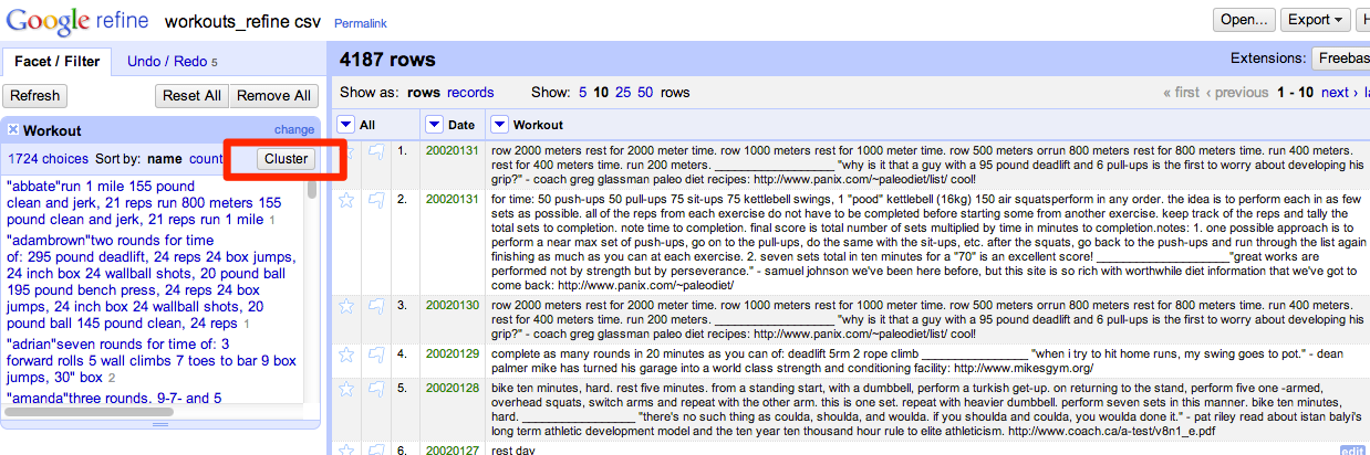
Open Refine has other methods to merge this sort of data and the option you pick depends on the problem at hand. For our case, the ‘fingerprint’ and ‘ngram-fingerprint’ techniques work quite well.

The tool forces you to go over each cluster it finds to merge, which is great. We only want to merge items that truly mean the same thing.

Next, clean up your data for the usual suspects:

Creating Derived Data

When you have data in one column that needs to be split into multiple columns or vice-versa, depending on the problem, you can either use Open Refine or Pandas.

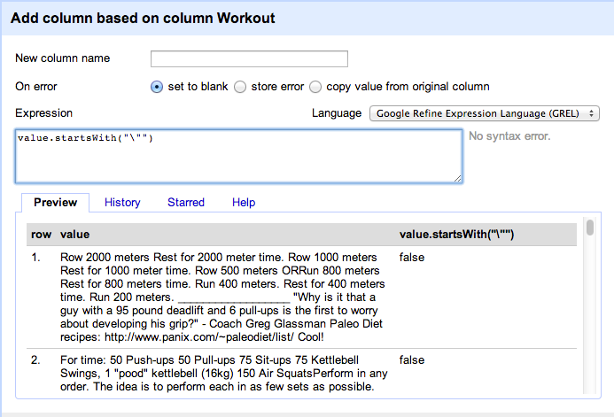
Some of the workouts on Crossfit.com are quite hard. These are usually Hero WODs (WOD stands for Workout of the day) or Benchmark WODs. The Hero WODs are named after fallen soldiers in war and benchmark workouts are have girl names and allow you to benchmark yourself over time. I wanted to see if there is an variance in the number of such workouts, year over year.

I noticed that all hero and benchmark workouts begin with double quotes. I created a derived boolean column out of the workout columns using the GREL syntax as below :

Now let’s import the data back into Pandas to generate some more derived columns.

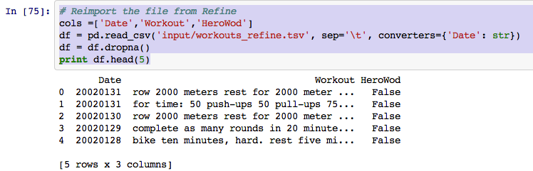
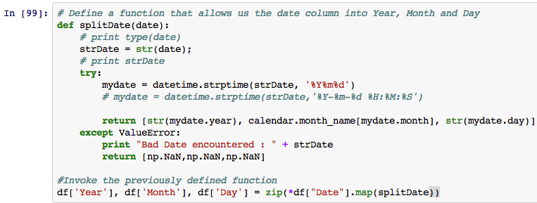
The date column is not very useful in this case if we want to perform any time series analysis. So let’s go ahead and split that into Year, Month and Day using Pandas.

Now our data is starting to look a little better.

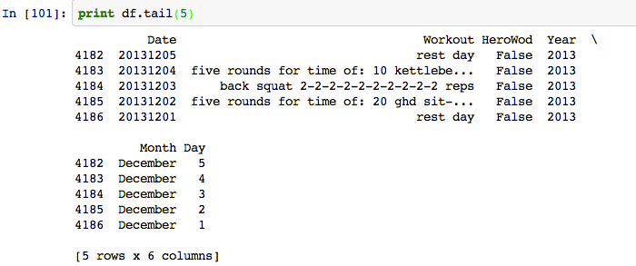
As you can see, the possibilities to derive and combine columns are endless.

Perform Sanity Checks

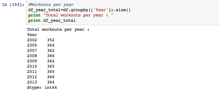
When dealing with unstructured data, like data scrapped from the web, it’s important to perform basic sanity checks. Especially with time series data, you want to make sure you have data for all time buckets. Let’s ‘Group By’ year to get the workout counts:

Let’s create a simple histogram with year buckets to ensure we have all the data points.

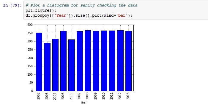
As you can see, we have fewer workouts for the years 2003, 2004, 2006 - so let’s get rid of that data from our dataframe.

Real world data is messy and uncomfortable. Start getting used to it and find ways to normalize data that is available. We will ignore this step for this post, to keep it simple.

Analyzing your Data

Here is where the real fun begins. You have clean data and all the columns you need. Let’s ask some interesting questions:

Has there been an increase or decrease in the number of 'hard' workouts?

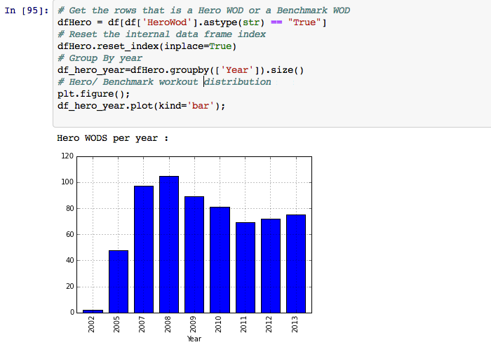
The direct answer to the question is neither. There was a peak in 2008 and ever since, the number trended down until 2011 and then picked up again in 2012.

The workouts shown in 2002 are outliers. They just happened to be workouts that started with double quotes. Ignoring that, we can tell that the Hero workouts / Benchmark workouts first started to appear in 2005 in our data. Going back and looking at the years of data we ignored (because of incomplete data), the first Hero WOD was posted on the 15th of July on 2004.

Comparing this data with the number of fallen soldiers (below) in the Iraq war, you notice a laggard correlation between the two data sets. Especially the data between 2007 and 2009.

Source : Wikipedia

This could very well be a case where we are looking too closely for an answer and there might be no relation at all. If you force data to find relations, you will most probably be able to do it - but it’ll be wrong. This concept translates nicely to the concept of overfitting a model in machine learning but let’s dive into that another day.

With Crossfit's popularity, have there been fewer rest days programmed every year?

We can solve this problem for the occurrence of the keyword ‘Rest Days’ in the workout column. We can bucket these occurrences by year and see a trend over time.

Let’s write a quick function that returns a series of the occurrence of a term in a data frame, grouped by year.

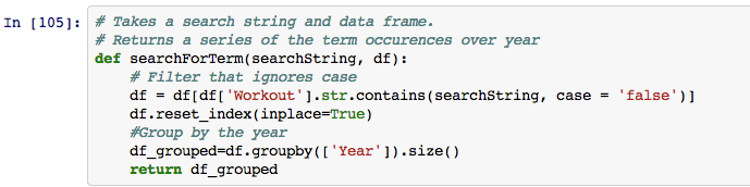
Using this function, we can pass in the search term to see the occurrences.

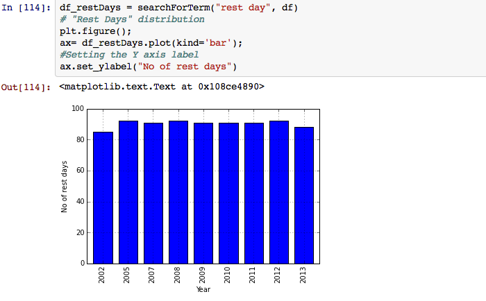
I was surprised to see that there was no real differences in the number of rest days programmed per year. The rest day schedule has been quite consistent and the programming itself is not completely ‘random’.

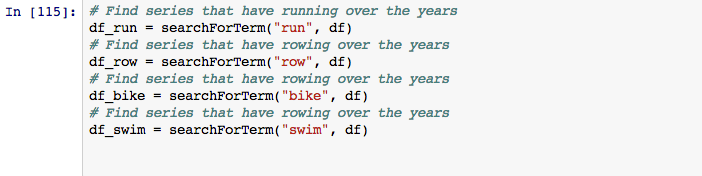
How many workouts have "cardio" involved? What is the trend?

Traditional cardio can be running, swimming, rowing and biking. We can make use of the previous search function we wrote to tabulate the occurrences of corresponding cardio exercises.

We concatenate all these dataframes into one dataframe which allows us to represent them as a stacked bar. A stacked bar is quite useful in comparing items placed in a time series.

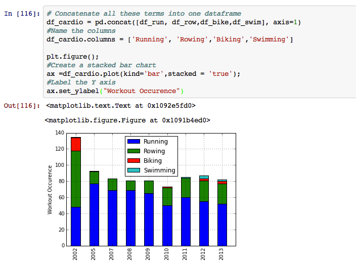
There are a couple of neat observations we can make from this bar chart:

1. Year 2002 was when rowing was first becoming popular and clearly the excitement is apparent in the workouts as well.
2. Swimming was never part of the workouts until the year 2011.
3. Biking was huge in 2002 and had completely died out by 2009, but is making a return again.
4. There has been a steady decrease in the number of running workouts and a steady increasing of rowing workouts again.

The list goes on…

A lot of different questions can be answered with this dataset and all the techniques we covered here. If you have interesting questions or get stuck trying to solve for a question, just let me know and I will be happy to assist.

There are a lot of unknown unknowns out there and exploratory data analysis allows you to make them known knowns. Don’t be afraid to explore them!

I love exploring data. Nothing explains it more than this quote.

“Fall in love with some activity, and do it! Nobody ever figures out what life is all about, and it doesn't matter. Explore the world. Nearly everything is really interesting if you go into it deeply enough. Work as hard and as much as you want to on the things you like to do the best. - Richard Feynman

As always, you can find the code and the IPython Notebook on Github here.